You know that, right now, “pandas” is the most popular open-source dataframe library in the world of Data Science. It has made in-memory analysis and in-memory processing of small to medium-sized 2D columnar data simple and fast. Not only in DS, but my observation also says that people use pandas extensively in other disciplines of SE as well – development, analytics, ML, infra, testing and you name it – wherever there are proper use cases to deal with a moderate pool of data efficiently and reliably. It, along with other dataframe libraries, has largely solved various problems related to data reading/writing, organising, wrangling, cleansing, manipulating, aggregating, analysing and visualisation.
Two limitations that pandas have:
1. It does not handle huge datasets where the size exceeds the available RAM (out-of-memory or OOM datasets)
2. It runs its queries on a single available CPU core in a single-thread
So, it does not utilise the power and capability of all the CPU cores available in the machine. The “Dask” dataframe library managed to somewhat solve these problems by writing wrappers on top of pandas, combining the in-memory pandas dataframes (partitioned along the index) and it is capable of distributing queries to multiple cores in parallel from underlying pandas’ single-threads.
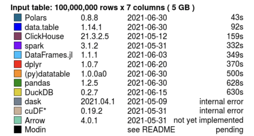
The lesser-known “polars” library has started to gain popularity now. It is another dataframe library and an in-memory query engine that was open-sourced a few years back. Unlike Dask, it does not depend on the pandas dataframe at all and has its implementation written from scratch (in Rust language). Its big advantage is that it utilises all the available cores and performs parallel multi-threaded execution after optimising the queries, making it blazingly fast and memory-efficient. There are multiple ways that polars perform query optimisation. The difference between performance and speed of execution between pandas and polars, for a dataset with a significant number of records, is pretty remarkable.
You can see below the performance benchmark observation done by H2O.ai for a task involving the “join” operation with “5GB” of columnar data:
(Something needs to be noted here: As I write this, the very recent version of pandas (v2.0.0) has provided the support of Apache Arrow backend for dataframe data. That means, it now has APIs to support data types representation for all data types – int, float, string, datetime with timezone, categories, other custom data types etc, along with existing APIs based on NumPy arrays. NumPy does have some known issues with certain datatypes like strings/date-times/custom data types and dealing with missing values).
Brief Intro to polars
The polars library has been written in Rust language. But it has provided bindings for Python and Node.js, enabling us to use polars in all these 3 languages. Under the hood, the library data structure is using “Apache Arrow Columnar format” as the memory model, following the Apache Arrow specification. This makes the data load-time, in-memory computation and usage very efficient. Polars has expressive, clear and strict declarative APIs for the users. They are called “expressions” and are always preferred to be used for almost all the use cases, to make full use of polars’ capabilities.
Working with polars – the basics
Let’s see how we can use start using polars python. You can use JS and Rust, but the APIs will obviously be different. I will talk about the python binding.
Install the polars package using pip:
pip install polarsSince the associated polars Rust binaries are pre-built in this package (in the form of compiled executable files), we don’t need to compile them separately to start using polars in Python.
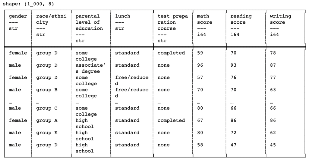
We can start by reading a fictional dataset (“Student performance prediction” dataset from Kaggle). The data is loaded into an excel file named “Students.xlsx”. As per Kaggle, this fictional dataset contains information on the performance of high school students in mathematics, including their grades and demographic information. To learn about polars, you can try using other supported formats like parquet, CSV and JSON of other datasets as well.
import polars as pl
df_pl = pl.read_excel("Students.xlsx")
print(df_pl)
Execution of the above lines will do a pretty print of the resultant dataframe object by displaying the column names, along with the datatypes (something we haven’t seen in pandas), as headers and the corresponding records of data below it. One thing to notice here is that, unlike pandas, polars does not use the concept of “indexing” and hence we will not see an index column at the start.
Some basic operations in polars have the same expression as pandas, like below:
print(df_pl.head()) # shows the first 5 rows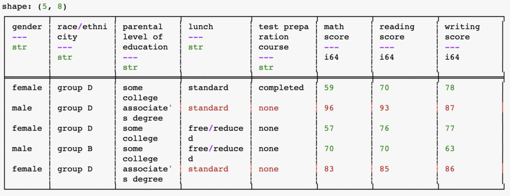
print(df_pl.tail()) # shows the last 5 rows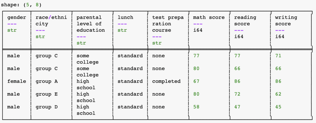
print(df_pl.describe()) # shows summary statistics of dataframe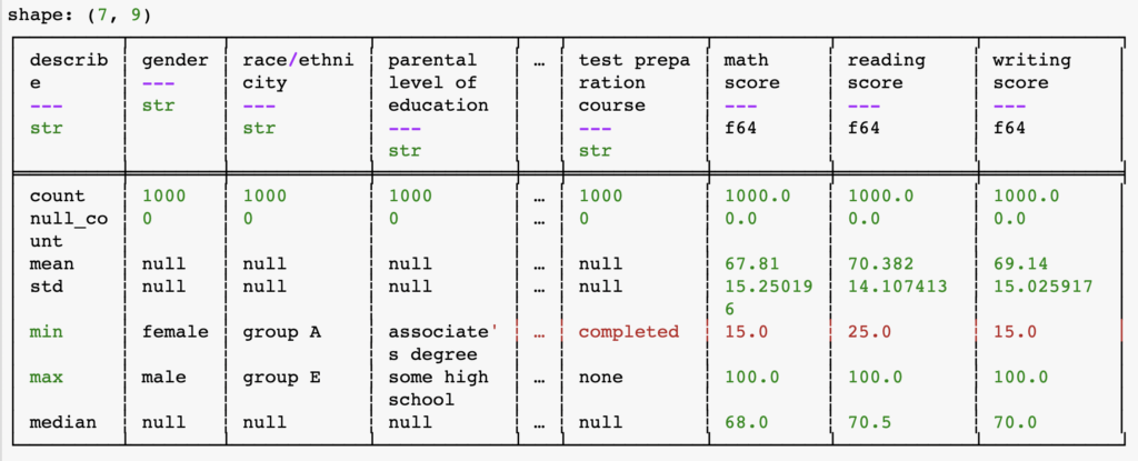
But the interesting parts start after that.
Working with polars – the “expressions”
To put it in simple words,
expressions in polars = building blocks of queries in polars
The polars expressions will help us to create simple to complex queries to load and fetch data.
1. select (displays columns)
Like SQL’s select, we can use polars’ “select” expression to select and display column data from the dataframe by mentioning the column names inside it.
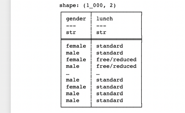
print(df_pl.select(pl.col(["gender", "lunch"])))
# OR
print(df_pl.select([pl.col("gender"), pl.col("lunch")]))
The above two lines select multiple columns using as list and positional arguments respectively.
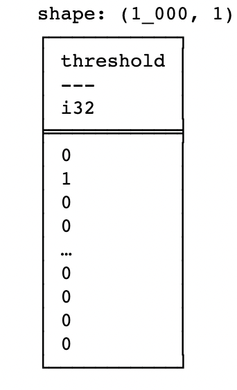
print(df_pl.select(threshold=pl.when(pl.col("math score") > 90).then(1).otherwise(0)))The above line uses keyword argument (“threshold“) to name the expression input after applying the logic and inserting values in it.
After navigating through the source code, I found that internally the “select” method of the “DataFrame” class in the “dataframe.frame” module of Polars’ python wrapper performs lazy loading and then passes the arguments to its “_from_pydf” classmethod which constructs and returns a Polars DataFrame from FFI (Foreign Function Interface) PyDataFrame object obtained from the Rust built-in. (I don’t know Rust language so could not deep-dive into the algorithm written inside it. But it will be something that will be on my radar to know).
Since I mentioned the term “lazy loading“, there is something you need to know at this point.
In polars, there are 3 strategies to load data into machine memories:
1) Eager loading
e.g. the action that is happening in the “read_excel” method. Internally, this read_excel method converts XLSX to CSV, then the CSV is parsed, and the subsequent loading strategy loads the entire dataset to the memory in a continuous way using an expensive “rechunk” operation and it then returns the appropriate DataFrame object at the end of it. The “pandas” library always performs eager loading for its queries. But polars has two other loading strategies too, to improve the query performance.
2) Semi-lazy loading
This strategy loads data into memory in chunks and performs the required operations after loading each chunk.
3) Lazy loading
In our previously mentioned “select” command example, for lazy loading, the “lazy()” method (of the “DataFrame” class in the “dataframe.frame” module of Polars’ python wrapper) instructs polars to hold on to the execution for subsequent queries. At the end, all the queries are collected and optimised by the “collect()” method which then performs eager loading, executes and collects the resultant DataFrame before returning it.
Below is the return statement for the “select” method in the “DataFrame” class
return self._from_pydf(
    self.lazy()
    .select(exprs, *more_exprs, **named_exprs)
    .collect(no_optimization=True)
    ._df
)
Source code wise, the “lazy()” method returns an object of the “LazyFrame” class which is a blueprint of a Lazy computation graph/query against the invoking DataFrame. Its “select” method then selects columns from the LazyFrame and returns a LazyFrame object. This returned LazyFrame object then calls its “collect” method to collect the result into a DataFrame object and returns it. As you might have noticed above, the value of “no_optimization” parameter of the “collect” method is turned True. What it does is – it turns off certain query optimization techniques like predicate_pushdown, projection_pushdown, slice_pushdown and common_subplan_elimination.
2. filters (creates a dataframe subset as per condition)
Below is a “filter” command that is operating on the dataframe and is filtering out rows based on a predicate expression (a boolean expression that returns either “True” or “False”) that evaluates to a Boolean series. Here, the predicate expression is: if the “math score” column value of the dataset is less than 30 and also the “reading score” column value of the dataset is greater than 50, return “True”, else return “False”.
df_pl.filter((pl.col("math score") <= 30) & (pl.col("reading score") >= 50))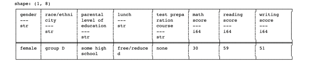
In this case, also, similar lazy loading takes place in the DataFrame class’ “filter” method.
return self._from_pydf(
    self.lazy()
    .filter(predicate)
    .collect(no_optimization=True)
    ._df
)
3. with_columns (creates new columns for analysis)
Following is an example of “with_columns” expression that appends 10 to the existing values of the “math score” column and displays them in a newly created column named “Increased math score“. If a column with the same name as the alias name exists, then the new column will replace the existing one.
df_pl = df_pl.with_columns((pl. col("math score") + 10).alias("Increased math score"))print(df_pl.select(pl. col(["math score", "Increased math score"])))

# OR, both the statements can be combined and written as:

print(df_pl.with_columns((pl. col("math score") + 10).alias("Increased math score")).select(pl. col(["math score", "Increased math score"])))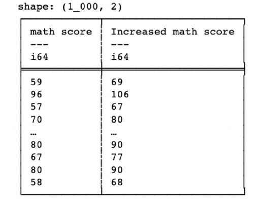
Let’s now see how can we integrate a visualization library (“plotly“) with “polars” and generate useful visualizations of our dataset.
For that, we need to install plotly and import plotly.express module
pip install plotlyimport plotly.express as pxWe will create 3 plots of the dataset:
1) A bar chart
2) A 2D scatter plot
3) A 3D scatter plot
To create the bar chart, let’s write a couple of lines:
fig1 = px.bar(df_pl.to_pandas(), x="parental level of education", color="parental level of education",
              color_discrete_sequence=["red", "blue", "green", "purple", "gray", "turquoise"])
fig1.show()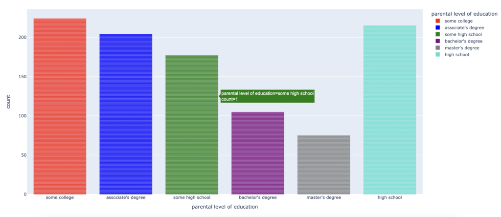
The chart shows the distribution of “parental level of education” values against the count. Hovering the mouse over the chart will dynamically display the distribution throughout the x-axis and the y-axis.
To create the 2D scatter plot, we will use the below 4 lines:
fig2 = px.scatter(df_pl.to_pandas(), x="math score", y="reading score", color="writing score", range_color=[0, 150])
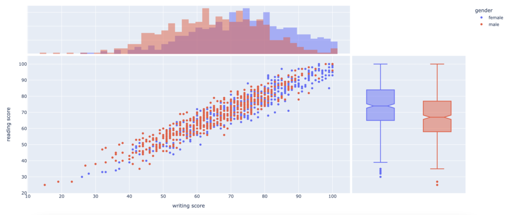
fig3 = px.scatter(df_pl.to_pandas(), x="writing score", y="reading score", color="gender", marginal_x="histogram",
marginal_y="box")
fig2.show()
fig3.show()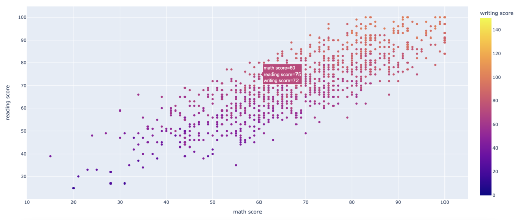
The first scatter plot shows the distribution of “math score” (on the x-axis), “reading score” (on the y-axis) and “writing score” (as colour distribution)
The second scatter plot shows the distribution of “writing score” (on the x-axis), “reading score” (on the y-axis) and “gender” (as colours distribution). In addition, it also shows a histogram along the x-axis and a box plot along the y-axis.
To create the 3D scatter plot, we will write and execute the below 2 lines:
fig4 = px.scatter_3d(df_pl.to_pandas(), x="writing score", y="reading score", z="gender", color="gender")
fig4.show()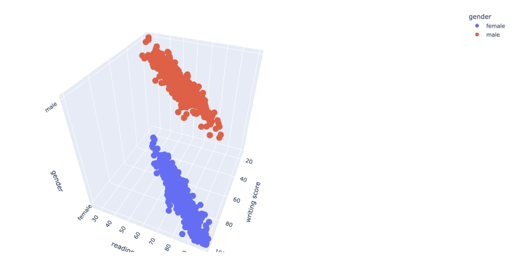
As you can see, polars’ integration with plotly is pretty smooth and other visualization libraries will hopefully also work without any problem. Let me know if you come across any library for which you are facing integration problems.
I hope you liked this article. Do subscribe to my newsletter if you have not done already and also share the information with your colleagues, friends and connections.
As always – keep learning, and keep sharing.