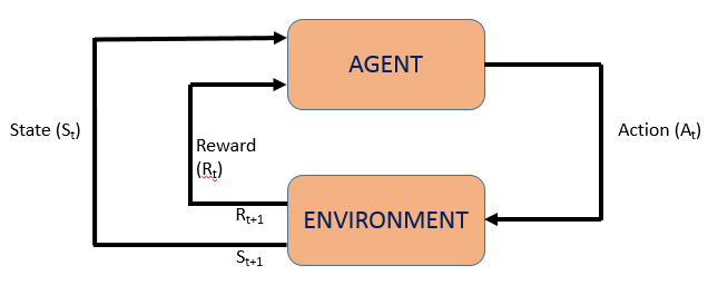
Reinforcement Learning is a machine learning technique in which the machine learning models learn from a series of decisions and employs trial-and-error mechanism to come up with a solution to problems in complex interactive environments. In a broader perspective, it is an artificial intelligence mechanism concerned with how software ought to take actions so as to maximize the notion of cumulative delayed reward. For example, training AI machines to perform tasks such as Walking, Running of Jumping.
The main idea behind reinforcement learning is based on the concepts of exploration of new territories and utilization of present knowledge to make decisions. It is also sometimes known as Online Learning and is used to solve interacting problems where the data observed up to time t1 is considered to decide which action is needed to be taken at time (t1 + 1). Desired outcomes deliver the model with “rewards” and undesired outcomes provide “penalties” to the model. The model begins to learn from this Trial-and-Error mechanism using feedback from its own actions and experiences. In the absence of existing training data, the model learns from its own experience and collects training examples by itself using the Trial-and-Error method with an aim to maximize the total reward. The model might start from random trials during the initial stages, learn from the given rewards or penalties and then start to exhibit sophisticated skills.
Reinforcement Learning is studied in many disciplines like economics, operations research, game theory, information theory, statistics, and genetics and in lot more.
There are some terms which are associated with Reinforcement Learning. They are –
agent (the decision making model)
environment (the place where the agent learns and makes decisions)
action (collection of actions taken by the agent)
state (agent’s current situation in the environment)
policy (method to map agent’s state to agent’s action)
reward (prize in the form of scalar value provided by the environment to the agent in case of correct decision taken)
value (Future reward that an agent would receive by taking an action in a particular state)
function approximators (refers to the problem of inducing a decision tree or neural nets function from the training examples collected by the agent).
Markov Decision Processes (MDP)
Markov Decision Processes or MDP are the Mathematical frameworks that can describe the interactive environments in the Reinforcement Learning processes. In mathematical terms, they are probabilistic models for sequence decision problems, where states can be perceived exactly and the current state and action selected determine a probabilistic decision on the upcoming future states. They consist of a set of finite environment States (S), a set of Actions A(S) for each state, a real valued Reward Function R(S) and a Transition Model P(S’, S|A). Almost all the Reinforcement Learning problems can be formalized using MDPs.
In this tutorial, we will discuss two popular Reinforcement Learning Algorithms:
1) Upper Confidence Bound
2) Thompson Sampling
But before diving into the algorithms directly, let’s first try to understand about the Multi-Armed Bandit Problem.
Multi-Armed Bandit Problem
In mathematical terms, a Multi-Armed Bandit problem (also called K/N-armed Bandit Problem) is a classic probabilistic Reinforcement Learning problem in which a limited set of resources must be allocated between alternative choices in a way that will maximize their reward gain. Each choice’s features are partially known at the time of allocation and may become well understood as time passes by or by allocating resources to the choice.
The name comes from imagining a gambler, in front of multiple slot machines in a casino (each machine is considered as “one-arm bandit”). The gambler has to decide which slot machines to play, how many times to play on each machine, which order to play them and whether to continue with the present machine or to try a different one to get the maximized chances of his gain. The probability distribution for the reward corresponding to each machine is different and is unknown to the gambler. As the gambler receives feedback about which machine- arms have the highest expected payout, he increases his proportion of trials with the higher expected payout machine-arms. The aim is to balance choosing the highest expected payout “exploitation” with receiving sufficient information “exploration” and find the arm with the highest expected payout. The Bandit algorithms are used in a lot of research projects like Clinical Trials, Network Routing, Online Advertising and Game Designing.
The most widely used solution method to the Multi-Armed Bandit Problems is Upper Confidence Bound (UCB) which is based on the principle of optimism in the face of uncertainty, that is, the more uncertain we are about a machine-arm, the more important it becomes to explore that machine-arm.
UPPER CONFIDENCE BOUND (UCB)
UCB is a deterministic algorithm which helps us selecting the best machine-arm based on a confidence interval in the multi-armed bandit problem. UCB is a deterministic algorithm meaning that there is no factor of uncertainty or probability. UCB focuses on exploration and exploitation based on a confidence boundary that the algorithm assigns to each machine on each round (when the gambler pulls the machine-arm) of exploration.
Consider there are 5 slot machines that the gambler has decided to play with – S1, S2, S3, S4 and S5. UCM will help us to devise a sequence of playing the machines in a way to maximize the reward gain from the machines.
Step1: Each machine is assumed to have a uniform Confidence interval and a success distribution.
Step2: The person picks up a random machine to play and all the machines are having the same Confidence Intervals at this point.
Step3: Based on whether the machine gave a “reward” or “penalty”, the Confidence Interval shifts either towards or away from the actual success distribution.
Step4: Based on the current calculated Upper Confidence Bounds of each of the machines, the one with the highest is chosen to explore in the next round.
Step5: Repeat Step3 and Step4 until there are sufficient observations to determine the UCB of each machine. The one with the highest UCB is the machine with the highest success rate.
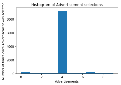
Let’s consider a dataset (WebsiteAds) consisting of 10 different advertisements. The goal of the UCB algorithm will be to find out the most clicked advertisement by the website visitors, that is, it will be trying to find out the advertisement with the maximum UCB. Let’s now see the code implementation in Python:
# Upper Confidence Bound Reinforcement Learning

# Import the required libraries and the collected dataset
import pandas as pd
import math
import matplotlib.pyplot as plotter
collectedDataset=pd.read_csv('WebsiteAds.csv')

# Implement the UCB algorithm in the collected dataset

NumberOfRounds=10000
NumberOfAds=10
ads_selected=[]
numbers_of_selections=[0]*NumberOfAds
sums_of_rewards= [0]*NumberOfAds
total_reward=0
for n in range(0,NumberOfRounds):
  ad=0
  max_upper_bound=0
  for i in range(0,NumberOfAds):
    if(numbers_of_selections[i]>0):
        average_reward=sums_of_rewards[i]/numbers_of_selections[i]
        delta_i=math.sqrt(3/2*math.log(n+1)/numbers_of_selections[i])
        upper_bound=average_reward+delta_i
    else:
        upper_bound=1e400
    if upper_bound > max_upper_bound:
        max_upper_bound=upper_bound
        ad=i
  ads_selected.append(ad)
  numbers_of_selections[ad]=numbers_of_selections[ad]+1
  reward=collectedDataset.values[n,ad]
  sums_of_rewards[ad]=sums_of_rewards[ad]+reward
  total_reward=total_reward+reward

# Visualize the Results
plotter.hist(ads_selected)
plotter.title('Histogram of Advertisement selections')
plotter.xlabel('Advertisements')
plotter.ylabel('Number of times each Advertisement was selected')
plotter.show()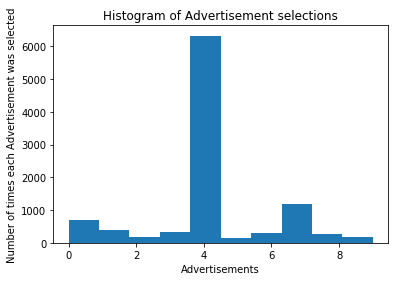
THOMPSON SAMPLING
Thompson Sampling (also known as Posterior Sampling/Probability Matching)is a Probabilistic Reinforcement Learning algorithm that follows exploration and exploitation to maximize the cumulative rewards obtained by performing an action by an agent in a complex environment. The algorithm uses Probabilistic Distribution and Bayes’ Theorem to generate success rate distributions.
Thompson Sampling algorithm can successfully handle the Multi-Armed Bandit Problem discussed above by making use of Probability Distribution and Bayes’ Rule to predict the success rates of each Slot machine.
Thompson Sampling Intuition
All the slot machines are assumed to have uniform probability distributions of success and reward. For each slot machine observation and reward, a new distribution gets generated with success probabilities for each machine. More observations are made based on these prior probabilities for each round and the success distributions are updated. In this way, after sufficient number of observations, each machine will have its own success distribution. The person can then choose the one machine out of all the other machines to get the maximized reward gain.
Let’s us now implement the Thompson Sampling algorithm in Python for the same WebsiteAds dataset. You can the find the dataset here.
# Thompson Sampling Reinforcement Learning

# Import the required libraries and the collected dataset
import pandas as pd
import random
import matplotlib.pyplot as plotter
collectedDataset=pd.read_csv('WebsiteAds.csv')

# Implement the Thompson Sampling Algorithm on the collected dataset
NumberOfRounds=10000
NumberOfAds=10
ads_selected=[]
numbers_of_rewards_1=[0]*NumberOfAds
numbers_of_rewards_0=[0]*NumberOfAds
total_reward=0
for n in range(0,NumberOfRounds):
  ad=0
  max_random=0
  for i in range(0,NumberOfAds):
    random_beta=random.betavariate(numbers_of_rewards_1[i]+1,numbers_of_rewards_0[i]+1)
    if random_beta > max_random:
        max_random=random_beta
        ad=i
  ads_selected.append(ad)
  reward=collectedDataset.values[n,ad]
  if reward==1:
    numbers_of_rewards_1[ad]=numbers_of_rewards_1[ad]+1
  else:
    numbers_of_rewards_0[ad]=numbers_of_rewards_0[ad]+1
  total_reward=total_reward+reward

# Visualize the Results
plotter.hist(ads_selected)
plotter.title('Histogram of Advertisement selections')
plotter.xlabel('Advertisements')
plotter.ylabel('Number of times each Advertisement was selected')
plotter.show()