As discussed earlier in the Introduction section of this Machine Learning tutorial, Unsupervised Learning is a machine learning method which learns through observation and finds structures in the data without getting the help of training data to train itself. Clustering (also known as Cluster Analysis) can be defined as an Unsupervised Machine Learning technique which groups a set of data points in such a way that the data points in the same group (cluster) are more similar to each other than to those in other groups (clusters). Clustering is not about any specific algorithm, rather it is an analysis technique which can be achieved with the help of various algorithms differing significantly in their understanding of what constitutes a cluster and how to efficiently find them.
The main aim of using Clustering algorithms is to segregate data with similar behavior and assign them into “Clusters”. Suppose, you are running an online business and you want to segregate your customers into 5 clusters based on some of their behaviors. This data insight will help you to understand the different types of customers and you can then come up with more customer-focused business strategies. How you choose to group them will help you to understand more about them as individual customers. When we apply Clustering Algorithms on the data, unexpected things can suddenly come up like structures, clusters and groupings which we would have never thought of otherwise.
Clustering algorithms can be applied to many fields like:
Biology: Grouping of animals and plants based on their features
Insurance: Grouping policy holders with high average claim cost or to identify frauds
Earthquake Prediction: Clustering earthquake epicenters to identify potential earthquake zones.
Marketing: Grouping customers according to their properties, salary or purchase history
Documents: Clustering documents based on similar words
Genetics: Clustering DNA sequences based on edit distance
Web: Segmenting users based on activities on website, application or platform
Inventory: Grouping inventory based on sales activity or manufacturing metrics
Some of the popular clustering methods include
Centroid-based Clustering (e.g. K-Means Clustering)
Connectivity-based/Hierarchical Clustering
Density-based Clustering
Distribution-based clustering etc.
Let’s now try to understand how the K-Means Clustering algorithm works.
K-MEANS CLUSTERING
K-Means Clustering is an Unsupervised Machine Learning Clustering technique which can be used to find clusters in unlabeled data (that is, data without defined categories/classes) based on feature similarity. The number of clusters is represented by the variable “K”. The algorithm works iteratively to assign each data point to one of K-groups based on the features that are provided.
Each ClusterCentroid is a collection of feature values which define the resulting clusters. Observing the centroid feature weights can be used to qualitatively interpret what kind of group each cluster represents. Once the algorithm has been modeled and run and the clusters are defined, any new data point can then be easily assigned to the correct cluster according to its features.
K-Means Clustering Steps
The K-Means clustering uses Iterative Refinement to produce the final outcome. The inputs to the algorithm are the number of clusters (K) and an unlabeled dataset (collection of features for all the data points).
Step1: Choose the number of clusters, that is, the value of “K”
Step2: Select at random K centroids, which can either be randomly generated or randomly selected from the dataset.
Step3: Assign each data point from the dataset to its closest Centroid. This results in the formation of K number of clusters.
Step4: Compute and place the new centroid for each cluster.
Step5: Reassign each data point from the dataset to the newly formed centroid which is closest to it. If any assignment took place at this step, go to Step4 and repeat the process until no assignment takes place.
Step6: Model is ready
Let’s now use K-Means Clustering Algorithm to create a model in order to cluster customers from the OnlineBusinessCustomers dataset. You can find the dataset here. Following is the model implementation in Python:
# K- means Clustering

# Import the required libraries and the collected dataset
import pandas as pd
import matplotlib.pyplot as plotter
collectedDataset = pd.read_csv('OnlineBusinessCustomers.csv')
X = collectedDataset.iloc[:, [3, 4]].values

# Use the Elbow Method to find out the optimal number of clusters
from sklearn.cluster import KMeans
wcss = [] # Within Cluster Sum of Squares
for i in range(1,11):
    kmeans=KMeans(n_clusters=i,init='k-means++',max_iter=300,n_init=10,random_state=0)
    kmeans.fit(X)
    wcss.append(kmeans.inertia_)
plotter.plot(range(1,11),wcss)
plotter.title('The Elbow Method')
plotter.xlabel('Number of Clusters')
plotter.ylabel('WCSS')
plotter.show()

# Apply the k-means clustering model to the collected dataset
kmeans=KMeans(n_clusters=5,init='k-means++',max_iter=300,n_init=10,random_state=0)
Y_kmeans=kmeans.fit_predict(X)

# Visualize the Clusters (for 2-D Clustering)
plotter.scatter(X[Y_kmeans==0,0],X[Y_kmeans==0,1],s=100,c='red',label='Cluster 1')
plotter.scatter(X[Y_kmeans==1,0],X[Y_kmeans==1,1],s=100,c='blue',label='Cluster 2')
plotter.scatter(X[Y_kmeans==2,0],X[Y_kmeans==2,1],s=100,c='green',label='Cluster 3')
plotter.scatter(X[Y_kmeans==3,0],X[Y_kmeans==3,1],s=100,c='cyan',label='Cluster 4')
plotter.scatter(X[Y_kmeans==4,0],X[Y_kmeans==4,1],s=100,c='magenta',label='Cluster 5')
plotter.scatter(kmeans.cluster_centers_[:,0],kmeans.cluster_centers_[:,1],s=300,c='yellow',label='Centroids')
plotter.title('Clusters of Online Business Customers')
plotter.xlabel('Annual Income (k$)')
plotter.ylabel('Spending Score (1-100)')
plotter.legend()
plotter.show()

# Visualize the Clusters with category names given (for 2-D Clustering)
plotter.scatter(X[Y_kmeans==0,0],X[Y_kmeans==0,1],s=100,c='red',label='Careful')
plotter.scatter(X[Y_kmeans==1,0],X[Y_kmeans==1,1],s=100,c='blue',label='Standard')
plotter.scatter(X[Y_kmeans==2,0],X[Y_kmeans==2,1],s=100,c='green',label='Target')
plotter.scatter(X[Y_kmeans==3,0],X[Y_kmeans==3,1],s=100,c='cyan',label='Careless')
plotter.scatter(X[Y_kmeans==4,0],X[Y_kmeans==4,1],s=100,c='magenta',label='Sensible')
plotter.scatter(kmeans.cluster_centers_[:,0],kmeans.cluster_centers_[:,1],s=300,c='yellow',label='Centroids')
plotter.title('Clusters of Online Business Customers')
plotter.xlabel('Annual Income (k$)')
plotter.ylabel('Spending Score (1-100)')
plotter.legend()
plotter.show()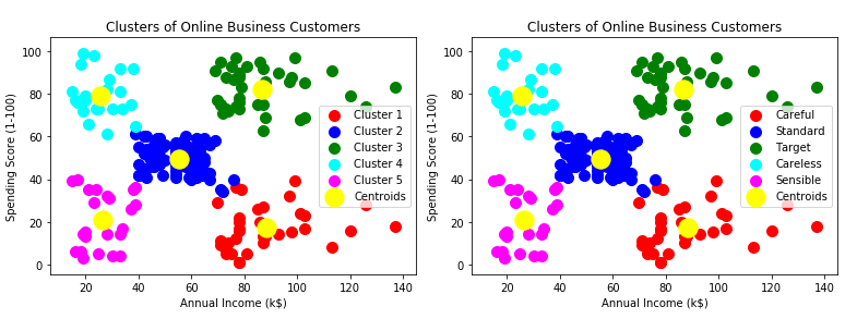
HIERARCHICAL CLUSTERING
Hierarchical Clustering or Hierarchical Cluster Analysis is an Unsupervised Machine Learning Clustering algorithm which creates clusters of similar data by initially treating each data point as a separate cluster. So, at its initial step it will form “N” number of clusters for “N” number of data points. The Hierarchical Clustering technique is basically divided into 2 types:
1) Agglomerative (Building Up) technique
2) Divisive (Building Down) technique
Agglomerative (Building Up) technique:
Here, each data point is considered to be an individual cluster. At each iteration of this technique, similar clusters merge with other clusters until one cluster or “K” clusters are formed.
Steps to perform Agglomerative Hierarchical Clustering:
Step1: Make each data point a single-point cluster. Thus, “N” number of data points correspond to “N” number of clusters
Step2: Take the 2 closest data points/clusters and make them one cluster. There are “N-1” number of clusters now.
Step3: Take the 2 closest clusters and join them to form a single cluster. This now results in “N-2” number of clusters.
Step4: Repeat Step3 until only a single cluster remains
Step5: Model is ready
The distance between the data points can be calculated based on their Euclidean distance (discussed in the CLASSIFICATION section of this tutorial).
The distance between the clusters can be calculated by taking either of the following ways:
– Finding the distance between the closest data points
– Finding the distance between the furthest data points
– Finding the average distance
– Finding the distance between the Centroids of the clusters
Dendrogram
Dendrograms are tree-like diagrams which act like memories of the Hierarchical Clustering algorithm depicting the hierarchical relationship between the data points. It records the sequences of data point/cluster merges or splits. Following is a pictorial representation of a Dendrogram:
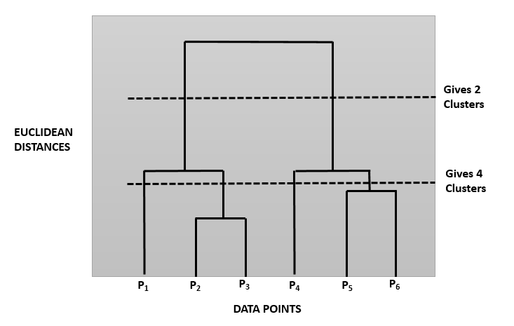
The height of the bar in this Dendrogram depicts the Euclidean Distance between 2 data points which are forming the cluster. Creation of Hierarchical Clustering Dendrogram usually consists of two important steps:
– Setting the Euclidean Distance Threshold (also known as the Dissimilarity Threshold)
– Number of Clusters = Number of perpendicular lines that cross the Euclidean Distance Threshold line. In this diagram, for the top dotted line, the number is 2 and for the below dotted line, the number is 4.
Divisive (Building Down) technique:
Here, at first, all the data points are considered to be inside a single cluster. At each iteration of this technique, the data points, which are not similar, are separated from the cluster. Then each data point, which is separated, is considered to be an individual cluster. At the end of this iteration activity, we will be left with “N” number of clusters. This technique is rarely used in real life scenarios.
Though the Agglomerative technique is quite popular while dealing with Hierarchical Clustering problems, Hierarchical Clustering algorithm itself has some disadvantages with regards to Space and Time Complexity. The space required for this algorithm is very high when the number of data points are very high as we need to store the similarity matrix in the RAM. The space complexity is the order of the square of n. Space Complexity is given by the formula:
Space complexity = O(n²)
where, “n” is the number of data points.
The Time Complexity for this algorithm also becomes quite high since n number of iterations will be performed and for each iteration, the similarity matrix is needed to be updated and restored. Time Complexity is given by the formula:
Time complexity = O(n3)
where, “n” is the number of data points.
Hence, this clustering algorithm is not preferred to create model for huge dataset.
Let’s now use Hierarchical Clustering Algorithm to create a model in order to cluster customers from the OnlineBusinessCustomers dataset. You can find the dataset here. Following is the code implementation in Python:
# Hierarchical Clustering

# Import the required libraries and the collected dataset
import matplotlib.pyplot as plotter
import pandas as pd
collectedDataset = pd.read_csv('OnlineBusinessCustomers.csv')
X = collectedDataset.iloc[:,[3,4]].values

# Use Dendrogram to find out the optimal number of clusters
import scipy.cluster.hierarchy as sch
dendrogram=sch.dendrogram(sch.linkage(X,method='ward'))
plotter.title('Dendrogram')
plotter.xlabel('OnlineBusinessCustomers')
plotter.ylabel('Euclidean Distances')
plotter.show()

# Fit the Hierarchical Clustering Model to the dataset
from sklearn.cluster import AgglomerativeClustering
hc=AgglomerativeClustering(n_clusters=5,affinity='euclidean',linkage='ward')
Y_hc=hc.fit_predict(X)

# Visualize the clusters
plotter.scatter(X[Y_hc==0,0],X[Y_hc==0,1],s=100,c='red',label='Careful')
plotter.scatter(X[Y_hc==1,0],X[Y_hc==1,1],s=100,c='blue',label='Standard')
plotter.scatter(X[Y_hc==2,0],X[Y_hc==2,1],s=100,c='green',label='Target')
plotter.scatter(X[Y_hc==3,0],X[Y_hc==3,1],s=100,c='cyan',label='Careless')
plotter.scatter(X[Y_hc==4,0],X[Y_hc==4,1],s=100,c='magenta',label='Sensible')
plotter.title('Clusters of OnlineBusinessCustomers')
plotter.xlabel('Annual Income (k$)')
plotter.ylabel('Spending Score (1-100)')
plotter.legend()
plotter.show()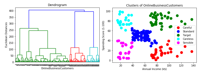
ASSOCIATION RULE LEARNING (ARL)
Association Rule Learning (ARL) or Association Rule Analysis is a rule-based Unsupervised Machine Learning technique which can be used to discover interesting relations between the items/elements/variables/features in a large dataset present in relational databases, transactional databases or any other data repository. Given a set of transactions, ARL aims to find the rules which will help us to predict the occurrence of a specific item based on the occurrences of the other items in the transaction.
Through the help of ARL we can uncover how items are associated to each other. The most popular application of ARL that you all are aware of – Recommendation Systems. Recommendation Systems take data about you, similar consumers and available products and use that to figure out what you might be interested in and therefore deliver promotional offers, coupons or suggestions based on the ARL.
Let us take an example:
The Association rule {Keyboard, Mouse} => {Mouse-Pad} found in the sales data of a digital store would indicate that if a customer buys a “Keyboard” and a “Mouse” together, then they are likely to buy a “Mouse-Pad”. This kind of information becomes very useful and can be used to make decisions about marketing activities such as promotional pricing or product placements in the store.
In layman terms, Association Rule Learning is a very simple technique – “People who bought this also bought something”, “If this happened, then the following is likely to happen”. In an ARL, the “if” part if called antecedent/left-hand-side(LHS) and the “then” part is called consequent/right-hand-side(RHS).
ARL Intuition:
Let us consider the following data:
I = {i1, i2, i3 ……… in} -> Set of n binary attributes (items)
T = {t1, t2, t3 …….. tm} -> Set of m transactions (database)
Each transaction in the set T has a unique transaction ID and contains a subset of the items in the set I. The Association Rule can then be defined as follows:
X => Y
where X, Y is a subset of I
X = antecedent/left-hand-side(LHS)
Y = consequent/right-hand-side(RHS)
Following is a database table with 5 transactions and 5 items from a digital store:
| ID | Keyboard | Mouse | MousePad | Headphone | Laptop Stand |
| 1 | 1 | 1 | 0 | 0 | 0 |
| 2 | 0 | 0 | 1 | 0 | 0 |
| 3 | 0 | 0 | 0 | 1 | 1 |
| 4 | 1 | 1 | 1 | 0 | 0 |
| 5 | 0 | 1 | 0 | 0 | 0 |
The set of items (I) is I = {Keyboard, Mouse, Mousepad, Headphone, Laptop Stand}
Each entry value “1” means that the item is present in that particular transaction and “0” means it is not present. An Association Rule for the Digital Store can be:
{Keyboard, Mouse} => {MousePad}
which means that if Keyboard and Mouse are bought, customers also buy Mouse-Pad. In real life applications, ARL requires thousands of transactions in the databases before it can be considered statistically significant.
In order to select important rules from the set of all possible rules, different constraints are used. The best known constraints are:
1) Support
2) Confidence
3) Lift
Support
The constraint “Support”is an indication of how frequently does the item appear in the dataset. If we consider the Digital Store example, then the support is:
support(I) = (Number of transactions containing the item I)/(Total Number of Transactions)
In the example dataset, the itemset X= { Headphone, Laptop Stand} has a support of 1/5=0.2 since it occurs on 20% of all the transactions.
Confidence
The constraint “Confidence” is an indication of how often the rule has turned out to be true. Confidence is given by the formula:
confidence(l1 -> l2) = (Number of transactions containing the items l1 and l2)/(Number of transactions containing the item l1)
For the Digital Store example, the rule {MousePad, Mouse} => {Keyboard} has a confidence of 0.2 / 0.2 = 1.0 in the database, which means that for 100% of the transactions containing MousePad and Mouse, the rule is correct (100% of the times a customer buys MousePad and Mouse, Keyboard is bought as well).
Lift
The “Lift” of a rule is defined as the ratio of the observed support to that expected if the items l1 and l2 were independent.
lift(l1 -> l2) = (confidence(l1 –> l2))/support(l2)
With the Association Rule Learning knowledge at our disposal, let’s now explore the following Association Rule algorithms:
– Apriori Algorithm
– Eclat Algorithm
APRIORI ALGORITHM
The Apriori Algorithm is an Association Rule Learning algorithm which identifies the frequent individual items in the dataset of the transactional databases and extends them to larger and larger item sets as long as those item sets appear sufficiently often in the database. The algorithm’s name is “Apriori” because it uses prior knowledge of frequent itemset properties. This algorithm applies an iterative approach to mine frequent itemsets, where k-frequent itemsets are used to find k+1 itemsets.
The algorithm is very useful for effective Market Basket Analysis. It helps the customers to purchase items easily without any hassle thereby increasing the market sales.
An important concept in Apriori algorithm is the anti-monotonicity of the constraint Support. It is based on the assumption that:
– All subsets of a frequent itemset must be frequent
– For any infrequent itemset, all its supersets must be infrequent
Apriori Steps:
Let us now see how to implement Apriori algorithm on the below Digital Store dataset:
| ID | Keyboard | Mouse | MousePad | Headphone | LaptopStand |
| 1 | 1 | 1 | 1 | 0 | 0 |
| 2 | 0 | 1 | 1 | 1 | 0 |
| 3 | 0 | 0 | 0 | 1 | 1 |
| 4 | 1 | 1 | 0 | 1 | 0 |
| 5 | 1 | 1 | 1 | 0 | 1 |
| 6 | 1 | 1 | 1 | 1 | 1 |
Let us consider the Support Threshold to be 50%, that is, only those items are significant for which support is more than 50%.
Step1: Create a frequency table of all the items occurring in all the transactions.
| Item | Frequency (Number of Transactions) |
| Keyboard (K) | 4 |
| Mouse (M) | 5 |
| MousePad (MP) | 4 |
| Headphone (H) | 4 |
| Laptop Stand (LS) | 2 |
Step2: We have to consider only those elements for which the support is greater than or equal to the Support Threshold (50%). Hence, only those items are significant which occur in more than 3 transactions and such items are Keyboard(K), Mouse(M), MousePad(MP) and Headphone(H).
Step3: Create all possible pairs of these significant items without considering the order, that is, AB is same as BA. To do this, take the first item and pair it with all the others – KM,KMP,KH. Similarly, consider the second item and pair it with the succeeding items, that is, MMP, MH. All the pairs formed now are – KM,KMP,KH, MMP, MH,MPH.
Step4: Now count the occurrences of each pair in all the transactions.
| Itemset | Frequency (Number of Transactions) |
| KM | 4 |
| KMP | 3 |
| KH | 2 |
| MMP | 4 |
| MH | 3 |
| MPH | 2 |
Step5: Again only those itemsets are now important which cross the Support Threshold(50%) and they are KM,KMP,MMP and MH.
Step6: Now we want to look for a set of 3 items which are purchased together. We will use the itemsets found in Step5 and create a set of 3 items using the “Self Join”rule (which says that from the item pairs KM,KMP,MMP and MH we look for 2 pairs with the identical first letter)
– KM and KMP -> This gives KMMP
– MMP and MH -> This gives MMPH
Step7: Now we find the frequency of these 2 itemsets
| Itemset | Frequency (Number of Transactions) |
| KMMP | 3 |
| MMPH | 2 |
Again, only that itemset is now significant which crosses the Support Threshold(50%) and it is KMMP. Hence, the set of 3 items that are purchased most frequently is KMMP or {Keyboard, Mouse, MousePad}.
Let’s now see the Python implementation of Apriori Algorithm to optimize the sales of a grocery store. The dataset (OnlineGroceryStore), that we will be using, can be found here. Here, we will be using 2 Python files – one contains the implementation of the Apriori algorithm (apyori.py) taken from the Python repository website PyPi and on the other one we will write the Apriori code.
# This is the code inside the apyori.py file
"""
a simple implementation of Apriori algorithm by Python.
"""

import sys
import csv
import argparse
import json
import os
from collections import namedtuple
from itertools import combinations
from itertools import chain


# Meta informations.
__version__ = '1.1.1'
__author__ = 'Yu Mochizuki'
__author_email__ = '[email protected]'


################################################################################
# Data structures.
################################################################################
class TransactionManager(object):
    """
    Transaction managers.
    """

    def __init__(self, transactions):
        """
        Initialize.

        Arguments:
            transactions -- A transaction iterable object
                            (eg. [['A', 'B'], ['B', 'C']]).
        """
        self.__num_transaction = 0
        self.__items = []
        self.__transaction_index_map = {}

        for transaction in transactions:
            self.add_transaction(transaction)

    def add_transaction(self, transaction):
        """
        Add a transaction.

        Arguments:
            transaction -- A transaction as an iterable object (eg. ['A', 'B']).
        """
        for item in transaction:
            if item not in self.__transaction_index_map:
                self.__items.append(item)
                self.__transaction_index_map[item] = set()
            self.__transaction_index_map[item].add(self.__num_transaction)
        self.__num_transaction += 1

    def calc_support(self, items):
        """
        Returns a support for items.

        Arguments:
            items -- Items as an iterable object (eg. ['A', 'B']).
        """
        # Empty items is supported by all transactions.
        if not items:
            return 1.0

        # Empty transactions supports no items.
        if not self.num_transaction:
            return 0.0

        # Create the transaction index intersection.
        sum_indexes = None
        for item in items:
            indexes = self.__transaction_index_map.get(item)
            if indexes is None:
                # No support for any set that contains a not existing item.
                return 0.0

            if sum_indexes is None:
                # Assign the indexes on the first time.
                sum_indexes = indexes
            else:
                # Calculate the intersection on not the first time.
                sum_indexes = sum_indexes.intersection(indexes)

        # Calculate and return the support.
        return float(len(sum_indexes)) / self.__num_transaction

    def initial_candidates(self):
        """
        Returns the initial candidates.
        """
        return [frozenset([item]) for item in self.items]

    @property
    def num_transaction(self):
        """
        Returns the number of transactions.
        """
        return self.__num_transaction

    @property
    def items(self):
        """
        Returns the item list that the transaction is consisted of.
        """
        return sorted(self.__items)

    @staticmethod
    def create(transactions):
        """
        Create the TransactionManager with a transaction instance.
        If the given instance is a TransactionManager, this returns itself.
        """
        if isinstance(transactions, TransactionManager):
            return transactions
        return TransactionManager(transactions)


# Ignore name errors because these names are namedtuples.
SupportRecord = namedtuple( # pylint: disable=C0103
    'SupportRecord', ('items', 'support'))
RelationRecord = namedtuple( # pylint: disable=C0103
    'RelationRecord', SupportRecord._fields + ('ordered_statistics',))
OrderedStatistic = namedtuple( # pylint: disable=C0103
    'OrderedStatistic', ('items_base', 'items_add', 'confidence', 'lift',))


################################################################################
# Inner functions.
################################################################################
def create_next_candidates(prev_candidates, length):
    """
    Returns the apriori candidates as a list.

    Arguments:
        prev_candidates -- Previous candidates as a list.
        length -- The lengths of the next candidates.
    """
    # Solve the items.
    item_set = set()
    for candidate in prev_candidates:
        for item in candidate:
            item_set.add(item)
    items = sorted(item_set)

    # Create the temporary candidates. These will be filtered below.
    tmp_next_candidates = (frozenset(x) for x in combinations(items, length))

    # Return all the candidates if the length of the next candidates is 2
    # because their subsets are the same as items.
    if length < 3:
        return list(tmp_next_candidates)

    # Filter candidates that all of their subsets are
    # in the previous candidates.
    next_candidates = [
        candidate for candidate in tmp_next_candidates
        if all(
            True if frozenset(x) in prev_candidates else False
            for x in combinations(candidate, length - 1))
    ]
    return next_candidates


def gen_support_records(transaction_manager, min_support, **kwargs):
    """
    Returns a generator of support records with given transactions.

    Arguments:
        transaction_manager -- Transactions as a TransactionManager instance.
        min_support -- A minimum support (float).

    Keyword arguments:
        max_length -- The maximum length of relations (integer).
    """
    # Parse arguments.
    max_length = kwargs.get('max_length')

    # For testing.
    _create_next_candidates = kwargs.get(
        '_create_next_candidates', create_next_candidates)

    # Process.
    candidates = transaction_manager.initial_candidates()
    length = 1
    while candidates:
        relations = set()
        for relation_candidate in candidates:
            support = transaction_manager.calc_support(relation_candidate)
            if support < min_support:
                continue
            candidate_set = frozenset(relation_candidate)
            relations.add(candidate_set)
            yield SupportRecord(candidate_set, support)
        length += 1
        if max_length and length > max_length:
            break
        candidates = _create_next_candidates(relations, length)


def gen_ordered_statistics(transaction_manager, record):
    """
    Returns a generator of ordered statistics as OrderedStatistic instances.

    Arguments:
        transaction_manager -- Transactions as a TransactionManager instance.
        record -- A support record as a SupportRecord instance.
    """
    items = record.items
    for combination_set in combinations(sorted(items), len(items) - 1):
        items_base = frozenset(combination_set)
        items_add = frozenset(items.difference(items_base))
        confidence = (
            record.support / transaction_manager.calc_support(items_base))
        lift = confidence / transaction_manager.calc_support(items_add)
        yield OrderedStatistic(
            frozenset(items_base), frozenset(items_add), confidence, lift)


def filter_ordered_statistics(ordered_statistics, **kwargs):
    """
    Filter OrderedStatistic objects.

    Arguments:
        ordered_statistics -- A OrderedStatistic iterable object.

    Keyword arguments:
        min_confidence -- The minimum confidence of relations (float).
        min_lift -- The minimum lift of relations (float).
    """
    min_confidence = kwargs.get('min_confidence', 0.0)
    min_lift = kwargs.get('min_lift', 0.0)

    for ordered_statistic in ordered_statistics:
        if ordered_statistic.confidence < min_confidence:
            continue
        if ordered_statistic.lift < min_lift:
            continue
        yield ordered_statistic


################################################################################
# API function.
################################################################################
def apriori(transactions, **kwargs):
    """
    Executes Apriori algorithm and returns a RelationRecord generator.

    Arguments:
        transactions -- A transaction iterable object
                        (eg. [['A', 'B'], ['B', 'C']]).

    Keyword arguments:
        min_support -- The minimum support of relations (float).
        min_confidence -- The minimum confidence of relations (float).
        min_lift -- The minimum lift of relations (float).
        max_length -- The maximum length of the relation (integer).
    """
    # Parse the arguments.
    min_support = kwargs.get('min_support', 0.1)
    min_confidence = kwargs.get('min_confidence', 0.0)
    min_lift = kwargs.get('min_lift', 0.0)
    max_length = kwargs.get('max_length', None)

    # Check arguments.
    if min_support <= 0:
        raise ValueError('minimum support must be > 0')

    # For testing.
    _gen_support_records = kwargs.get(
        '_gen_support_records', gen_support_records)
    _gen_ordered_statistics = kwargs.get(
        '_gen_ordered_statistics', gen_ordered_statistics)
    _filter_ordered_statistics = kwargs.get(
        '_filter_ordered_statistics', filter_ordered_statistics)

    # Calculate supports.
    transaction_manager = TransactionManager.create(transactions)
    support_records = _gen_support_records(
        transaction_manager, min_support, max_length=max_length)

    # Calculate ordered stats.
    for support_record in support_records:
        ordered_statistics = list(
            _filter_ordered_statistics(
                _gen_ordered_statistics(transaction_manager, support_record),
                min_confidence=min_confidence,
                min_lift=min_lift,
            )
        )
        if not ordered_statistics:
            continue
        yield RelationRecord(
            support_record.items, support_record.support, ordered_statistics)


################################################################################
# Application functions.
################################################################################
def parse_args(argv):
    """
    Parse commandline arguments.

    Arguments:
        argv -- An argument list without the program name.
    """
    output_funcs = {
        'json': dump_as_json,
        'tsv': dump_as_two_item_tsv,
    }
    default_output_func_key = 'json'

    parser = argparse.ArgumentParser()
    parser.add_argument(
        '-v', '--version', action='version',
        version='%(prog)s {0}'.format(__version__))
    parser.add_argument(
        'input', metavar='inpath', nargs='*',
        help='Input transaction file (default: stdin).',
        type=argparse.FileType('r'), default=[sys.stdin])
    parser.add_argument(
        '-o', '--output', metavar='outpath',
        help='Output file (default: stdout).',
        type=argparse.FileType('w'), default=sys.stdout)
    parser.add_argument(
        '-l', '--max-length', metavar='int',
        help='Max length of relations (default: infinite).',
        type=int, default=None)
    parser.add_argument(
        '-s', '--min-support', metavar='float',
        help='Minimum support ratio (must be > 0, default: 0.1).',
        type=float, default=0.1)
    parser.add_argument(
        '-c', '--min-confidence', metavar='float',
        help='Minimum confidence (default: 0.5).',
        type=float, default=0.5)
    parser.add_argument(
        '-t', '--min-lift', metavar='float',
        help='Minimum lift (default: 0.0).',
        type=float, default=0.0)
    parser.add_argument(
        '-d', '--delimiter', metavar='str',
        help='Delimiter for items of transactions (default: tab).',
        type=str, default='\t')
    parser.add_argument(
        '-f', '--out-format', metavar='str',
        help='Output format ({0}; default: {1}).'.format(
            ', '.join(output_funcs.keys()), default_output_func_key),
        type=str, choices=output_funcs.keys(), default=default_output_func_key)
    args = parser.parse_args(argv)

    args.output_func = output_funcs[args.out_format]
    return args


def load_transactions(input_file, **kwargs):
    """
    Load transactions and returns a generator for transactions.

    Arguments:
        input_file -- An input file.

    Keyword arguments:
        delimiter -- The delimiter of the transaction.
    """
    delimiter = kwargs.get('delimiter', '\t')
    for transaction in csv.reader(input_file, delimiter=delimiter):
        yield transaction if transaction else ['']


def dump_as_json(record, output_file):
    """
    Dump an relation record as a json value.

    Arguments:
        record -- A RelationRecord instance to dump.
        output_file -- A file to output.
    """
    def default_func(value):
        """
        Default conversion for JSON value.
        """
        if isinstance(value, frozenset):
            return sorted(value)
        raise TypeError(repr(value) + " is not JSON serializable")

    converted_record = record._replace(
        ordered_statistics=[x._asdict() for x in record.ordered_statistics])
    json.dump(
        converted_record._asdict(), output_file,
        default=default_func, ensure_ascii=False)
    output_file.write(os.linesep)


def dump_as_two_item_tsv(record, output_file):
    """
    Dump a relation record as TSV only for 2 item relations.

    Arguments:
        record -- A RelationRecord instance to dump.
        output_file -- A file to output.
    """
    for ordered_stats in record.ordered_statistics:
        if len(ordered_stats.items_base) != 1:
            continue
        if len(ordered_stats.items_add) != 1:
            continue
        output_file.write('{0}\t{1}\t{2:.8f}\t{3:.8f}\t{4:.8f}{5}'.format(
            list(ordered_stats.items_base)[0], list(ordered_stats.items_add)[0],
            record.support, ordered_stats.confidence, ordered_stats.lift,
            os.linesep))


def main(**kwargs):
    """
    Executes Apriori algorithm and print its result.
    """
    # For tests.
    _parse_args = kwargs.get('_parse_args', parse_args)
    _load_transactions = kwargs.get('_load_transactions', load_transactions)
    _apriori = kwargs.get('_apriori', apriori)

    args = _parse_args(sys.argv[1:])
    transactions = _load_transactions(
        chain(*args.input), delimiter=args.delimiter)
    result = _apriori(
        transactions,
        max_length=args.max_length,
        min_support=args.min_support,
        min_confidence=args.min_confidence)
    for record in result:
        args.output_func(record, args.output)


if __name__ == '__main__':
    main()
# Apriori Associate Rule Learning
# Import the required libraries and the collected dataset
import pandas as pd
collectedDataset = pd.read_csv('OnlineGroceryStore.csv', header = None)
onlineTransactions = []
for i in range(0, 7501):
onlineTransactions.append([str(collectedDataset.values[i,j]) for j in range(0, 20)])
# Train the Apriori algorithm on the dataset
from apyori import apriori
associationRules = apriori(onlineTransactions, min_support = 0.003, min_confidence = 0.2, min_lift = 3, min_length = 2)
# Visualize the results
associationRuleResults = list(associationRules)
output =[]
for i in range(0, len(associationRuleResults)):
output.append(['Rule:\t' + str(associationRuleResults[i][2][0][0]), 'Effect:\t' + str(associationRuleResults[i][2][0][1]),
'Support:\t' + str(associationRuleResults[i][1]), 'Confidence:\t' + str(associationRuleResults[i][2][0][2]),
'Lift:\t' + str(associationRuleResults[i][2][0][3])])ECLAT ALGORITHM
The word “ECLAT” stands for Equivalence Class Clustering and bottom-up Lattice Traversal. The ECLAT algorithm is a more modern, efficient, scalable and faster version of the Apriori algorithm since it imitates the Depth-First search of a graph unlike the Apriori algorithm which imitates the Breadth-First search of a graph. It represents the data in a vertical format and carries out a Depth-first search on the subset lattice and determines the support of itemsets by intersecting the transaction lists.
ECLAT Algorithm Intuition:
Consider the below table of transactions in a Digital Store:
| ID | Keyboard | Mouse | MousePad | Headphone | LaptopStand |
| T1 | 1 | 1 | 0 | 0 | 1 |
| T2 | 0 | 1 | 0 | 1 | 0 |
| T3 | 0 | 1 | 1 | 0 | 0 |
| T4 | 1 | 1 | 0 | 1 | 0 |
| T5 | 1 | 0 | 1 | 0 | 0 |
| T6 | 0 | 1 | 1 | 0 | 0 |
| T7 | 1 | 0 | 1 | 0 | 0 |
| T8 | 1 | 1 | 1 | 0 | 1 |
| T9 | 1 | 1 | 1 | 0 | 0 |
In each cell (i.j) of the above dataset, the value denotes whether the jth item is included in the ith transaction or not with the value 1 meaning true and 0 meaning false.
For k=1 and Minimum Support =2
| Item | TransactionID Set |
| Keyboard | {T1, T4, T5, T7, T8, T9} |
| Mouse | {T1, T2, T3, T4, T6, T8, T9} |
| MousePad | {T3, T5, T6, T7, T8, T9} |
| Headphone | {T2, T4} |
| LaptopStand | {T1, T8} |
Now, iterate on the function with increasing value of k until no more item-transaction id pairs can be combined
For k=2
| ItemSet | TransactionID Set |
| {Keyboard,Mouse} | {T1, T4, T8, T9} |
| {Keyboard,MousePad} | {T5, T7, T8, T9} |
| {Keyboard,Headphone} | {T4} |
| {Keyboard,LaptopStand} | {T1, T8} |
| {Mouse,MousePad} | {T3, T6, T8, T9} |
| {Mouse,Headphone} | {T2, T4} |
| {Mouse,LaptopStand} | {T1,T8} |
| {MousePad,LaptopStand} | {T8} |
For k=3
| ItemSet | TransactionID Set |
| {Keyboard,Mouse,MousePad} | {T8, T9} |
| {Keyboard,Mouse,LaptopStand} | {T1,T8} |
For k=4
| ItemSet | TransactionID Set |
| {Keyboard,Mouse,MousePad,LaptopStand} | {T8} |
Here, at this point there is no TransactionID Set to combine together. Since, we have considered the minimum support=2 hence, we can give the following recommendation table based on the ECLAT algorithm:
| Item Bought | Recommended Item |
| Keyboard | Mouse |
| Keyboard | MousePad |
| Keyboard | LaptopStand |
| Mouse | MousePad |
| Mouse | Headphone |
| Mouse | LaptopStand |
| {Keyboard,Mouse} | MousePad |
| {Keyboard,Mouse} | LaptopStand |
Let’s now see the Python implementation of the ECLAT Algorithm to optimize the sales of a grocery store. The dataset (OnlineGroceryStore) can be found here. Here, we will be using 2 Python files – one contains the implementation of the Apriori algorithm (apyori.py) taken from the Python repository website PyPi and on the other one we will write the ECLAT code which will use the apyori.py file
# Eclat Association Rule Learning

# Import the required libraries and the collected dataset
import pandas as pd
collectedDataset = pd.read_csv('OnlineGroceryStore.csv', header = None)
transactions = []
for i in range(0, 7501):
    transactions.append([x for x in collectedDataset.values[i] if str(x) != 'nan'])

# Train the Apriori on the dataset
# With no min confidence and lift, for Eclat
from apyori import apriori
rules = apriori(transactions, min_support = 0.004, min_confidence = 0, min_lift = 0)

# Visualize the results
eclatResults = list(rules)
# Sort by the support in decending order
eclatResults.sort(key=lambda tup: tup[1], reverse=True)
# Set the min length for the results
min_length = 2
eclatResults_list = []
for i in range(0, len(eclatResults)):
   if len(eclatResults[i][0]) >= min_length:
      eclatResults_list.append('RULE:\t' + str(eclatResults[i][0]) + '\nSUPPORT:\t' + str(eclatResults[i][1]))