Cluster bugs using ML (K-Means Clustering Algorithm) - A step-by-step approach

There are a few potential areas in the quality engineering space where applying Machine Learning concepts can help us get deep insights. It is not a necessity that only applied ML can bring an extensive understanding of those areas. Some solid plain engineering work can also achieve the same. But the existence of some libraries, used extensively for ML works, makes the work far easier.

One of those use cases is the “clustering” of software bugs found for a software product. It’s about understanding the nature of the bugs and then grouping them into different “clusters” (i.e. groups) based on some common characteristics. The concept can be applied by starting with a few features of the bugs (as shown in this article) and then can be extended to include multiple features. The more bug features are included, the better the groupings will be. The efficacy will also depend on the amount of data. The larger the dataset, the better. Collecting the data for only a few test cycles/sessions will not be that effective. My suggestion is to keep on collecting the data for every cycle/session, over a long period of time and keep on looking into what the algorithm result is telling you. The results can uncover some very useful information that is difficult to perceive with the naked eye.

Before starting, let’s first understand what is clustering in ML. “Clustering” (or Cluster Analysis) is an unsupervised machine learning technique that groups a set of data points in such a way that the data points in the same group (cluster) are more similar to each other than to those in other groups (clusters). Here, the term “unsupervised” means the model will be trained on unlabelled data without the supervision/help of human-labelled examples as the training set. Such kind of model usage becomes helpful when we want to discover patterns, relationships or structures in the collected data. The model will explore the collected data, learn and do these on its own, before segregating the data and putting them into clusters.

Let’s take the example of an imaginary bugs dataset defined by the equation:

import numpy as np
bug_data = np.random.rand(100, 2) * 4

These two lines generate a 2-dimensional NumPy array called “bug_data” with a shape of 100 rows and 2 columns. The array is filled with random values between 0 and 1, and these values are then multiplied by 4, resulting in a range between 0 and 4. Consider the two columns to be representative of some features related to the bugs like “Occurrence frequency” (or “Application Module/Component affected”) and “Bug Severity” respectively.

[Note: Instead of using this kind of random imaginary dataset, as a numpy array, you can replace this with your own bug dataset. You can put them into either a CSV file or Excel file, create a pandas dataframe out of them and then follow the remaining process, but the concept remains the same]

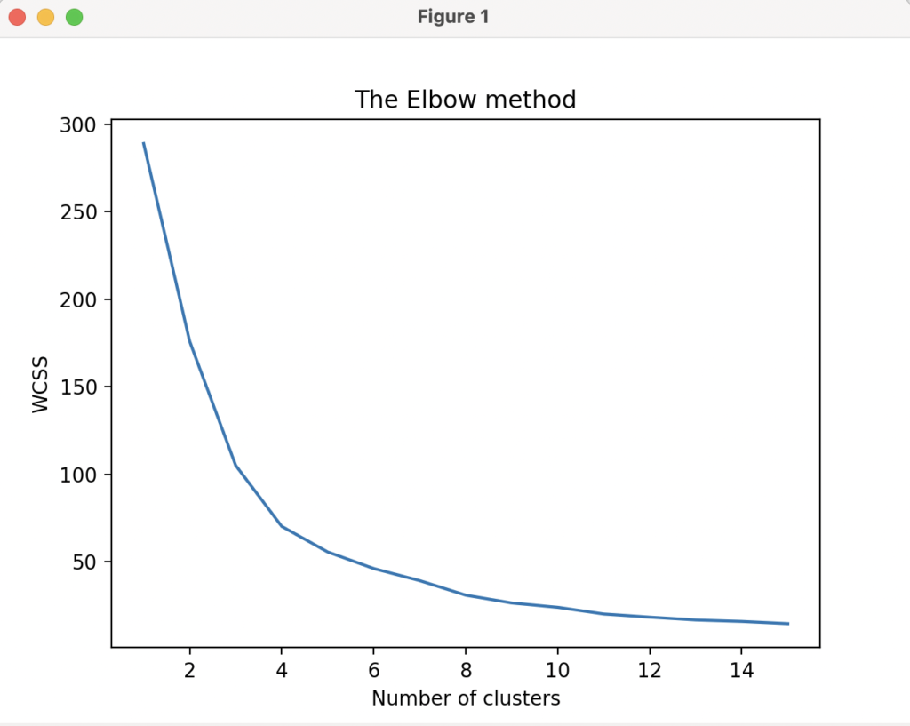
Next, we need to enable the model to determine, on its own, the optimal number of clusters that we have to use in the model. Here, the ML model algorithm that I am using is “K-means clustering” and the method to determine the number of clusters is “The Elbow method”.

import matplotlib.pyplot as plt
from sklearn.cluster import KMeans

wcss = []  # within cluster sum of squares
for i in range(1, 16):
    kmeans = KMeans(n_clusters=i, init="k-means++", max_iter=300, n_init=10, random_state=0)
    kmeans.fit(bug_data)
    wcss.append(kmeans.inertia_)
plt.plot(range(1, 16), wcss)
plt.title("The Elbow method")
plt.xlabel("Number of clusters")
plt.ylabel("WCSS")
plt.show()

I am importing two Python modules here (“matplotlib.pyplot” from the matplotlib library and “sklearn.cluster” from the scikit-learn library).

I created an empty Python list (“wcss”) which will represent the “within-cluster sum of squares”. This mathematical calculation/metric is used to evaluate the clustering results in the K-Means algorithm. Mathematically, it measures the sum of squared distances between each data point and the centroid of its assigned cluster.

Next, I initialised a KMeans object with some specific parameters like below:

n_clusters=i -> specifies the number of clusters to create. The value of i is determined by a the loop I am using (range(1, 16))

init=”k-means++” -> specifies the initialisation method for centroids

max_iter=300 -> specifies the maximum number of iterations for the K-means algorithm to converge.

n_init=10 -> specifies the number of times the algorithm will be run with different centroid seeds. The final result will be the best output in terms of WCSS

random_state=0 -> sets the random centroid seed for reproducibility

Then by using the below line, I am fitting the bug dataset to the initialised K-Means model.

kmeans.fit(bug_data)

The above line performs the actual clustering by assigning each data point to one of the clusters.

wcss.append(kmeans.inertia_)

Next, the above line calculates the WCSS metric (defined earlier) and adds the value to the previously declared “wcss” empty Python list. Here, “kmeans.inertia_” returns the WCSS value for the fitted model, which represents the sum of squared distances between each data point and its centroid.

The below lines will plot the data points and enable us to determine the value where the “elbow” seems to be breaking.

plt.plot(range(1, 16), wcss)
plt.title("The Elbow method")
plt.xlabel("Number of clusters")
plt.ylabel("WCSS")
plt.show()

That value will be the “number of clusters” that we have to use. Looking into the diagram here, that number seems to be “3”.

We need to use this cluster number (i.e. 3) for the subsequent actions of the model. For that we are declaring a variable (k) and initialising it with the value “3”

k = 3
kmeans = KMeans(n_clusters=k, random_state=0) 
kmeans.fit(bug_data)
labels = kmeans.labels_
centers = kmeans.cluster_centers_

kmeans = KMeans(n_clusters=k, random_state=0)

This line will initialise the K-means clustering model considering the cluster number as “3”

kmeans.fit(bug_data)

This line will fit the bug data to the K-means model

labels = kmeans.labels_

This line will get the cluster labels assigned to each bug

centers = kmeans.cluster_centers_

This line will help us to get the cluster centroids

To plot the formed clusters using pyplot, we can use the below lines (comments included):

plt.figure(figsize=(8, 6))

# Define marker styles and colors for each cluster
markers = ["o", "s", "^"]
colors = ["red", "blue", "green"]
for cluster_label in range(k):
    cluster_points = bug_data[labels == cluster_label]
    plt.scatter(cluster_points[:, 0], cluster_points[:, 1], marker=markers[cluster_label],
                color=colors[cluster_label])
plt.scatter(centers[:, 0], centers[:, 1], marker="x", s=200, c="black")
plt.xlabel("Bug Severity")
plt.ylabel("Occurrence Frequency")
plt.title("Bug Clustering for Bug Analysis")

# Create legend
legend_elements = [plt.Line2D([0], [0], marker=markers[i], color='w', markerfacecolor=colors[i], markersize=10)
                   for i in range(k)]
plt.legend(legend_elements, ['Cluster {}'.format(i + 1) for i in range(k)])
plt.show()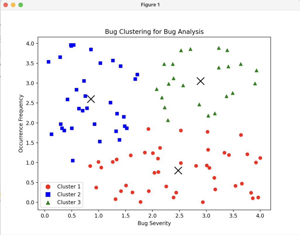

In some other article, I will try to cluster the same dataset using other Clustering techniques (Hierarchical, Density-based clustering, Topic modelling) and see how the plots will look like and which one out of these gives the best results.

Posts

Cluster bugs using ML (K-Means Clustering Algorithm) – A step-by-step approach